Vifm can show some statistics about an ongoing file operation and recently it was suggested to add an ETA there as well. I have an issue with ETAs because of how wrong they often are, so the plan was to find out what’s the best way to implement one before proceeding. Unfortunately, I wasn’t able to find anything useful that could aid in making the decision. I found a lot of frustration about ETAs similar to mine, but essentially no recommendations that were substantiated with anything tangible, so I decided to compare different ways to compute an ETA myself.
Alternatives
The only other test I’ve seen is here, but it compares two specific algorithms (by computing ratio of sums of absolute errors in a suspicious way) and each run produces different results because inputs are random. Not very useful.
Results
No need to postpone this until the very end. The benchmark itself is here under a very inventive name of etabench (this post corresponds to the state fixed at post branch). Results are:
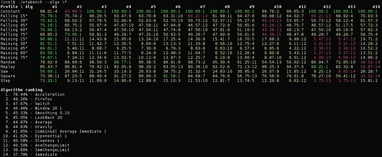
There is a column per algorithm and their order reflects result of the benchmark. Cells of the table indicate accuracy of an algorithm on that profile in percents relative to the ideal ETA for the profile. Numbers after a colon are ranks within a profile (if there is a tie, two results will have the same rank). Green means the best result in the row (so for a particular profile), red means the worst one and light yellow indicates everything in between.
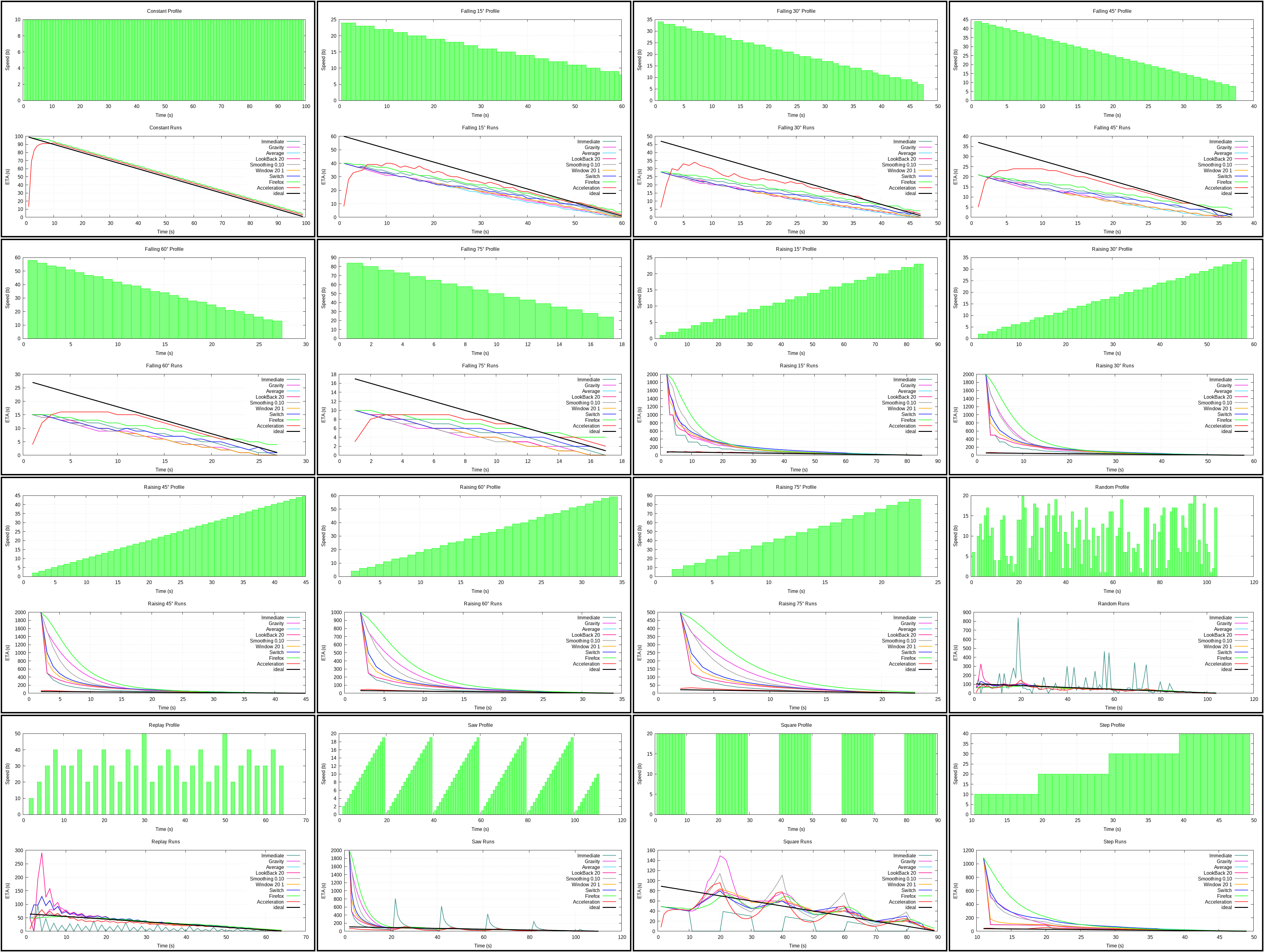
In a form of a plot results can be seen here (3.6 MiB). This includes only algorithms enabled by default and it’s already barely readable. Here and below plots won’t be embedded, because their file size is quite large and resolution is larger than 4000x3000, so scaled down versions are useless anyway.
Disclaimers
This is primarily targeting I/O operations in a file manager and results might be biased toward this particular usage as that’s the use case I’m thinking about.
I don’t know what I’m doing :) I don’t usually model and benchmark stuff, so mistakes are fairly possible.
I’m bad at math. Luckily, it’s not really needed in most cases, but I have a feeling that someone competent in math/statistics would be able to come up with better benchmark/algorithms. I had to make some calls for measuring similarity and if that’s really wrong, the whole benchmark is of no use. Really hoped to find some paper on ETA algorithms, but couldn’t and tend to think that I just failed to find it.
After seeing Acceleration algorithm being better than the rest, I dedicated quite a lot of time to improving it further. Other algorithms can probably be tuned to be better as well, although it’s unclear to what degree.
There were multiple occasions where I’ve messed up implementation of an algorithm in a way that significantly affected its ranking (both ways, by the way). Keep that in mind and take a look at the implementation before discarding it.
The Benchmark Setup
ETA function
This is a stateful function which is invoked with three arguments:
- Current progress.
- Total amount.
- Current (simulated) time.
Each call is expected to return a new ETA. Units used can be thought of as bytes (progress and amount) and seconds (time and ETA). Note that not all algorithms can be implemented like this. For example, an approach where total workload is split into separate tasks doesn’t fit into this scheme, more so if tasks can be run in parallel.
For convenience time starts at 0 and function is not called with current progress being zero (thus effectively excluding invocations with time equal zero as well) because no algorithm will be able to produce any meaningful ETA for this case. The time between invocations always grows by one. The state is reset before running an algorithm on a different profile.
There are two interesting state changes that every algorithm has to deal with:
- First call. Going from empty previous state to first non-empty state might need special handling.
- No progress. Speed dropping to zero can reset state to an empty one, freeze it or update it in some way. Then when it goes back to non-zero, behaviour of the first call can repeat or something entirely different can happen.
In both of these cases there is a transition to or from zero, both of which can require special handling. Depending on what’s done, user might have very different experience and final evaluation of the algorithm can also change quite dramatically for profiles with zeros.
Evaluation
Obviously, results are relevant only as long as simulation is not too different from a real word. This is achieved by running each algorithm on a set of profiles where transfer speed goes up or down differently and sometimes drops down to zero.
Total size of data transferred is the same for all algorithms and is 1000 by default. Changing it does affect results, but not too drastically (mostly equally bad algorithms swap places). One of the reasons for the changes is that profiles do not depend on the total size and can be quite small (like 10-20). In real world with larger files and larger speeds, results are expected to stay relevant as both are scaled proportionally. Smaller numbers in the benchmark allow keeping verbose output and graphs manageable.
My primary interest here is IO and it can be done on a single large file as well as on a large number of small ones and anything in between. Different profiles are supposed to take this into account and averaging them should provide an adequate score for an algorithm.
Similarity
Measured as a cosine similarity between ideal ETA and the one under the test. Both functions are non-negative and result is in the range [0; 1], which is convenient. There is however an issue however with normalization, interpretation here is that of an angle between two vectors, but angle doesn’t depend on the length of those vectors.
After looking at some alternatives and not finding a good pick I
ended up multiplying cosine similarity with a ratio like min/max where min
and max are smaller and greater integrals of the two ETAs. This way the more
different the two integrals, the smaller the similarity. It’s still not
perfect, but seems to work better than the other things I’ve tried.
Shape
Generally speaking, smoother ETA is better. Jumps are acceptable if their number is relatively small and the algorithm recovers from them fast enough. Wobbling can also be tolerated if it’s of a small enough magnitude.
This property, however, wasn’t measured in any way, although it is captured by the plots (when scale allows for it). Can probably compare slope of the measured algorithm to the slope of ideal ETA function, which is a line. Have yet to try this out.
Profiles
At the moment there are 16 profiles (half of them are variations on the same theme):
- Constant (fixed speed)
- Falling 15° (speed falls at 15 degrees)
- Falling 30° (speed falls at 30 degrees)
- Falling 45° (speed falls at 45 degrees)
- Falling 60° (speed falls at 60 degrees)
- Falling 75° (speed falls at 75 degrees)
- Raising 15° (speed raises at 15 degrees)
- Raising 30° (speed raises at 30 degrees)
- Raising 45° (speed raises at 45 degrees)
- Raising 60° (speed raises at 60 degrees)
- Raising 75° (speed raises at 75 degrees)
- Random (speed is generated pseudo-randomly with a fixed seed)
- Replay (speed variation is derived from a real-world data)
- Saw (speed goes up, drops to zero, then repeats)
- Square (speed is fixed, then zero for the same amount of time)
- Step (speed goes up in fixed period of time)
Profiles are depicted in plots, see links to them below if descriptions aren’t clear enough.
By the way, in case you are wondering why you were taught trigonometric functions, it’s so that you could implement those Falling/Raising profiles :)
Algorithms
Mind that since algorithms were tested using the benchmark they can be optimized for it. They also depend on its assumptions. You might have to do adjustments before using them in real life.
Names of the algorithms were picked to be reasonably short and descriptive enough for the purposes of viewing benchmarking results. Being too accurate and/or specific wasn’t a priority here.
More complicated algorithms often use simpler algorithms as their building blocks and then add some pre- and/or post-processing.
Another thing to keep in mind is that some algorithms have parameters and their performance depends on them. Using them in practice might require deriving those parameters based on the total.
At the time of writing of this post the benchmark included 14 algorithms.
Average (plot)
The #1 most obvious algorithm: use average speed to compute remaining time, where average speed is progress divided by elapsed time.
Terrible when speed actually increases, but nonetheless comes out in the middle of the scoring board, which is not that bad.
Immediate (plot)
The #2 most obvious algorithm: use immediate speed to compute remaining time, divide recent progress by the time it took to make it.
Has the same issue with the speed up as Average algorithm, but in addition to that can jump all over the place. Literally the worst one if time period used for computing speed is too short (every invocation in this case).
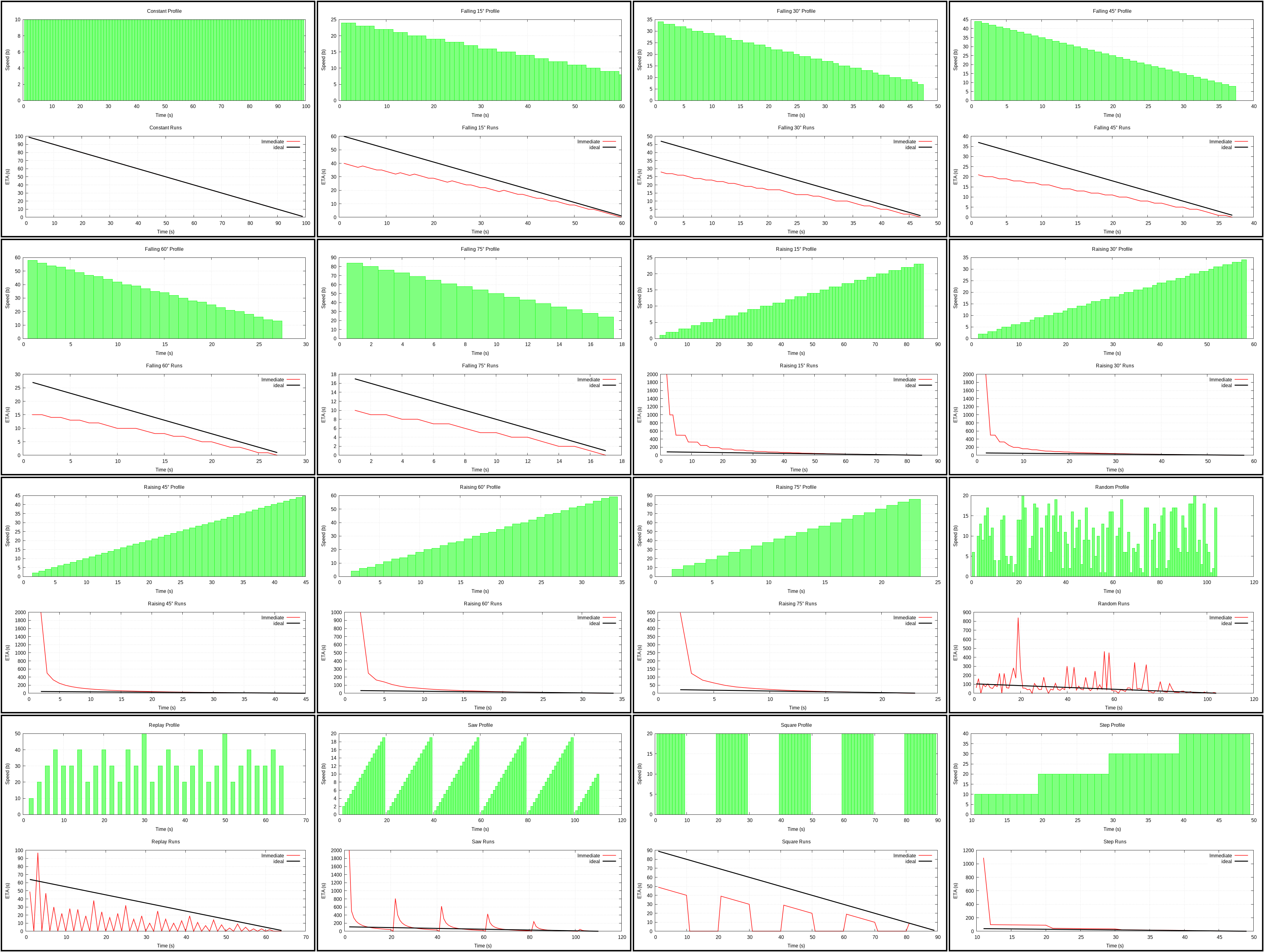
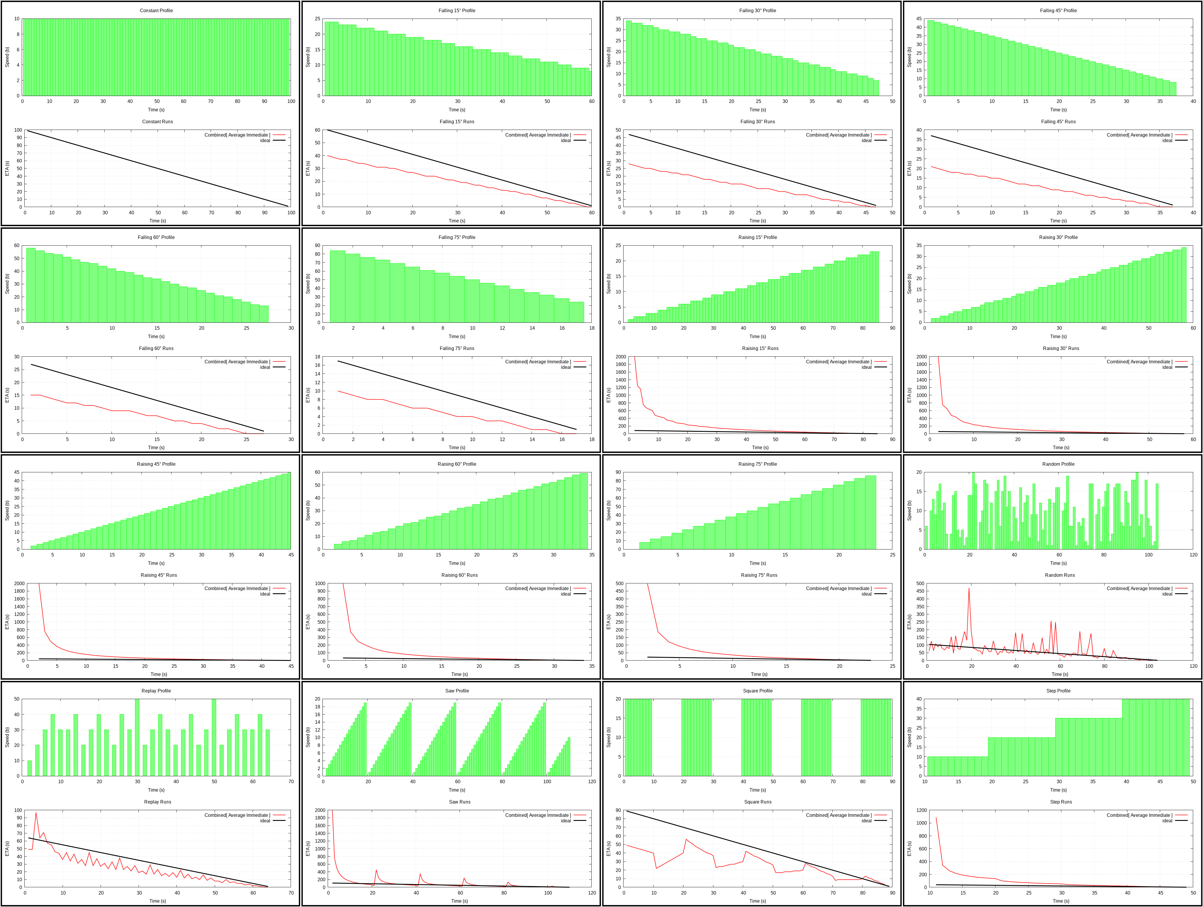
Combined Average and Immediate (plot)
On trying to come up with something better than the two previous algorithms, people suggest to just average them. Does it work? Not really.
At least with 0.5 weight for each, result is better than for Immediate and worse than Average. Just use Average instead.
ImmChangeLimit (plot) and AveChangeLimit (plot)
After looking at how crazy Immediate can get, I decided to clamp speed in order to stabilize it. Then I did the same for Average just for the symmetry.
It did smooth ETA quite nicely, the problem is that it made recovery from an initial jump awfully slow. As a result this is worse than Average and is technically better than Combined, but not really. Without preventing the jump, this is no good and reaction time to changes might generally be slow even after that (changing clamping limits to more than 2% can remedy some of it).
LookBack 20 (plot)
This is essentially Average algorithm that goes back at most N (20 in this
case) last seconds instead of going all the way to the beginning. Do not
confuse this for weighted average where every data point gives contribution,
here difference between an older moment and the current one is used to
approximate speed.
I’ve implemented this one as a different way to combine Immediate and Average algorithms. It actually does better than Average and even climbs up to the second place when the total grows. However, it still has that ugly spike at the beginning when the speed goes up.
Switch (plot)
Suggested here: use Average until 50% is reached, then assume that
remaining X percent will behave as previous X percent.
So first we have the same issues as with Average, which misbehaves at the start, then we use quite unjustified assumption about the future. It works similar to neighbouring algorithms above and below, but requires a more complicated implementation.
Window 20 1 (plot)
This is your weighted average (well, weight is 1, so it’s a regular average) of immediate speeds in the last 20 seconds.
Why weight of 1? Using different coefficients didn’t make it rank higher. Not that weights don’t matter, they just don’t seem to help if weighting is basically the only thing that happens.
Gravity (plot)
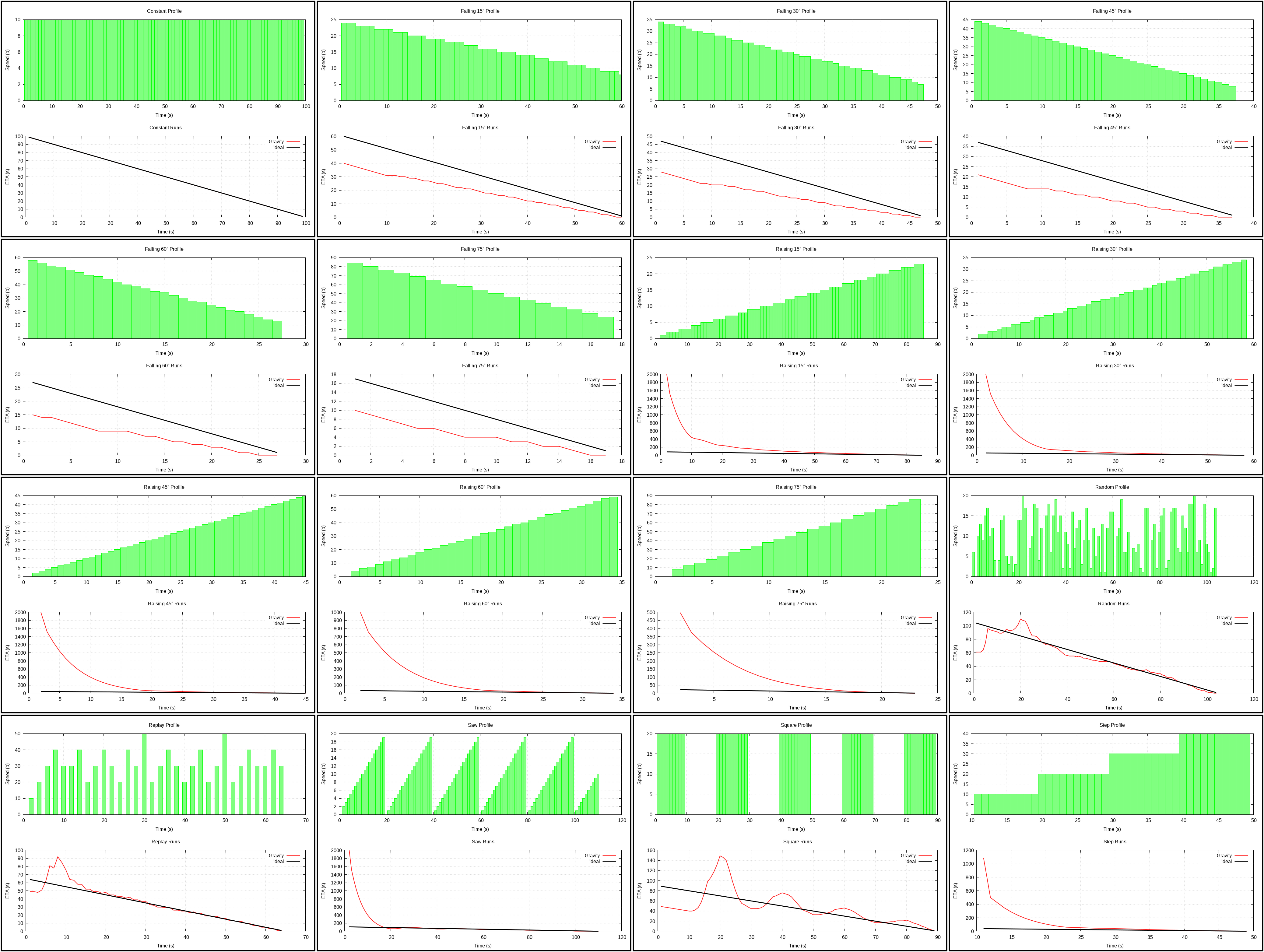
Based on this answer which offers an interesting idea for reducing jitter: modelling ETA as a heavy physical object. Current estimated speed is used to compute immediate remaining time estimate, which tells whether current time estimate should move up or down as if it were an object of a particular mass at a particular hight from the ground (hight is the difference between current and immediate time estimate).
Unfortunately it doesn’t seem to work particularly well in practice, scoring at the level of Average algorithms.
Smoothing 0.10 (plot)
Called this way because of the smoothing factor and it’s shorter than saying
exponential moving average. You obviously get different results for
different factor, but a value <= .2 seems like a popular choice and the one
which works quite well (I chose 0.10, because it worked better than 0.20).
It follows from the formula that the larger the factor the larger will be jumps on sudden changes, however the smaller the factor the bigger the error on the start (smaller estimated speed leads to huge ETA).
Scores a bit better than Average.
Exponential 1 (plot) and Slowness 1 (plot)
You can find nice description here (although that’s not the only place where exponential smoothing is described).
Both rank next to each other with Exponential being a bit better. Exponential is smoothing that uses 1/e as its coefficient. And it doesn’t seem to be a good choice for the coefficient.
Slowness sounds interesting, but acts weird. I don’t think I understood decay rate and how to pick it. The implementation might be wrong.
I didn’t bother implementing double exponential smoothing as I doubt it would work much better.
Firefox (plot)
Described here: smoothing of immediate speed with factor 0.1, then slowly adjusting previous ETA towards the newly computed one.
Similar to Average on the start. Because it changes slowly, it’s quite smooth. Quite good, but not without issues.
I like how smoothing is done with different factors depending on whether estimate grew or fell in the last computation.
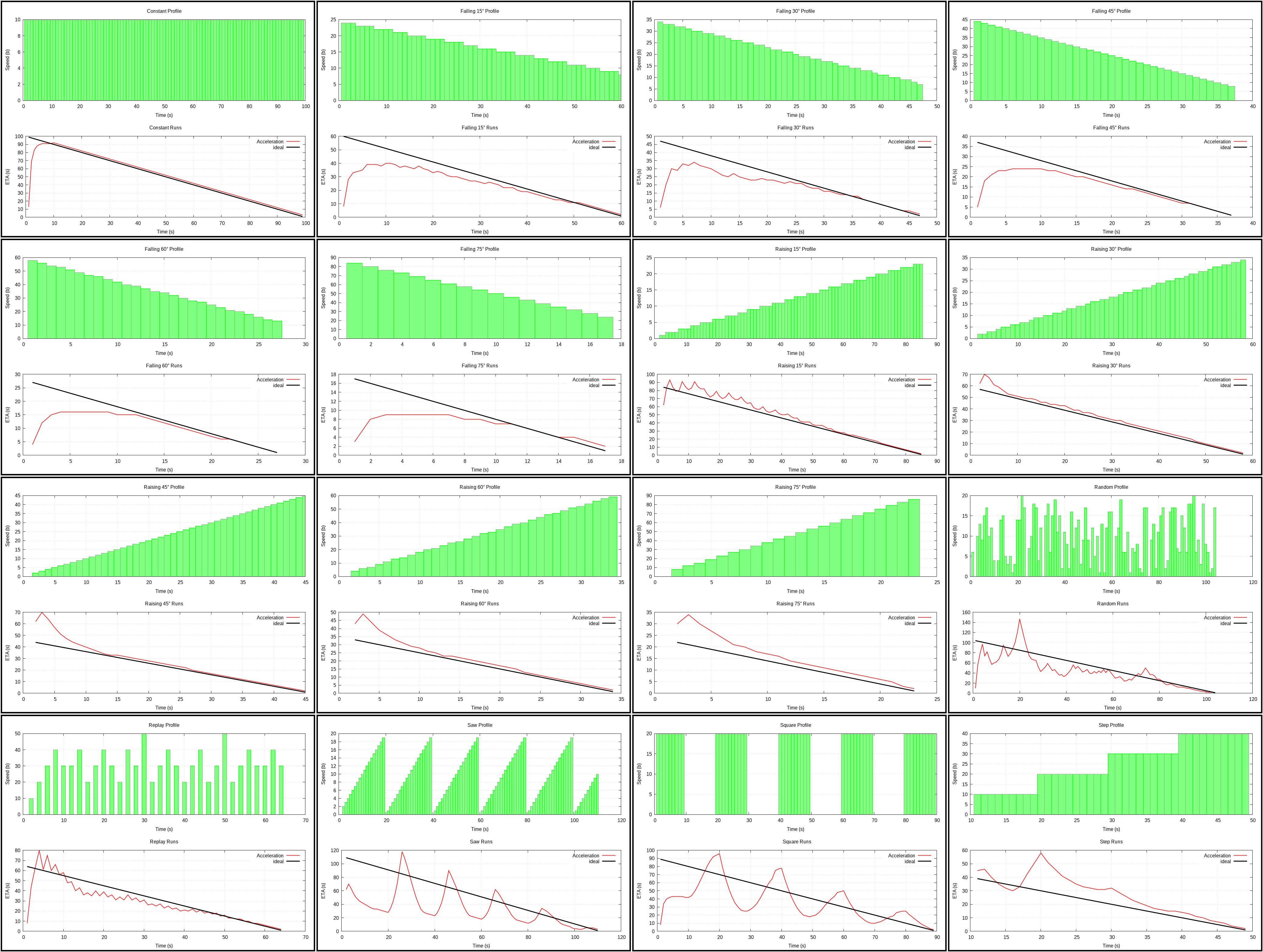
Acceleration (plot)
I was surprised this wasn’t suggested anywhere. We know issues of ETA with acceleration and deceleration, we know the speed, so why not compute how it changes and take it into account using a formula from the school?
Computing with acceleration is not always possible as complex numbers can appear. When speed drops to zero and stays there, this algorithm effectively freezes ETA computation. If there is speed, but no acceleration, have to resort to a regular computation without acceleration.
One of the reasons it has higher scores is that it’s overly conservative at the start where many other algorithms tend to produce huge estimates that then drop to more reasonable values. It does have a disadvantage of underestimating ETA at first, but it doesn’t take long to recover from that and on average this produces better results.
The damping is implemented in a way such that changes happen slower the more far apart old and new values are:
if (v != 0 && lastV != 0) {
    auto [minV, maxV] = std::minmax<float>(v, lastV);
    v = lastV + (v - lastV)*minV/maxV;
}
Interestingly, I tried plugging this into other algorithms, but it didn’t help there (e.g., in Average). This is probably because they don’t use acceleration. Here side-effect of starting computation is pushed from speed to acceleration, both are taken into account and factoring in acceleration actually decreases ETA (!), which is the opposite to the rest of the algorithms.
Eventually, I also added weighted average for immediate speed (applied before damping mentioned above; weights are 1, 2, 4, …) and ETA (weights are 1, 2, 3, …) to get smoother curve and improve the score of the algorithm even more.
Monte Carlo (not implemented)
Suggested here, but seems inappropriate for progress measurements unless the operation is rather stable (in which case simpler methods will do similarly well). If speed consistently goes up, down or significantly deviates from what was going on previously in any other way, the estimate computed via this method is likely to look just random.
Unused (so far) Ideas
Taylor Series
I had somewhat high hopes for this one, but still not sure if it can work (as mentioned above, I’m bad at math). Original idea was to have this as an evolution of Acceleration algorithm, which uses two derivatives of progress (speed and acceleration), but have more of them. As I understand, by reversing obtained series with fixed number of terms to get the value of an inverse function (which should be time) one can do this at least in some cases (can there be cases like negative discriminant in Acceleration?).
I think my initial attempt was just wrong at how it computed derivatives, so I might give it another try later.
Fitting
Curve fitting also comes to mind and not just to mine (couldn’t find where I saw it, should be in the sources), however as far as I remember it’s terrible in the corners and we’re talking about extending function in the future by a lot here. That said, it might generate useful results, I didn’t try it though.
Feedback Loop
The point is to determine error of the previous estimate and use that to correct the current one. Since we know how much time has passed, we can subtract it from the previous estimate and get a new expected one. Difference from that and a newly computed estimate can be used to improve the new estimate.
The ways in which such feedback could be incorporated vary.
This was temporarily used for Acceleration, but then got removed. Adding it helped at first, but turned out to be getting in the way after applying other changes. Still think that this can be useful in some cases.
This question mentions Kalman filter which seems to do something similar. However, it assumes Gaussian distributions of sources of random noise with zero mean, which doesn’t really sound like speed changes while copying files.
User Feedback
Knowing expected estimate and how things actually go, one could communicate level of accuracy to the user.
A variant of this was suggested in this StackOverflow answer as well as in several answers on this question. Surprisingly some people argue against displaying this information to the user, but they are probably the same people who give users no configuration options at all. I think an interval can be displayed to the user or can be determined and then used to increase ETA in the direction of its upper bound.
Varying Parameters
Another variation on feedback could involve tuning parameters on the go. For example, window size could be adjusted in response to speed changes. The longer the speed changes, the wider becomes the window, but when it becomes more stable (e.g., adjacent measurements don’t differ more than 5%), window size shrinks.
Weird Weighting
Make weights of averaged value proportional to the values? Would that help to dampen jumps?
Conclusions
Acceleration algorithm showed itself better than the rest in most cases. It’s not ideal, wobbles a bit and even jumps sometimes, but all in all it’s quite good in general.
Is Acceleration algorithm the best one can do? I doubt it. Although, I have to admit that 78% is pretty good (nearly twice better than the simplest implementations!). Even better ETA algorithms probably have an upper bound not too far away from that at least on this set of profiles. I’d expect those algorithms to use more derivatives or some other parameters of progress to make better estimates. You can read about discarding old rates and such to improve results or collecting stats from multiple runs, but not much on squeezing more out of already available data, which is where accuracy should come from.
The most important thing for me is that I now have means for comparing and testing of ETA algorithms and there is no need to rely on a gut feeling so much when implementing/adjusting ETA in Vifm or elsewhere.
Sources
I’ve spent quite a lot of time on this (maybe too much), did many searches (got few relevant results) and read through the links. Not everything is linked above as some things are just common knowledge or are mentioned somewhere but not actually explained. There is still a lot to try out and I’m done with this for now. In case anyone wants to give it a try or thinks I’ve missed something, below is a small tree of links that I’ve saved along with a bit of notes.
- https://stackoverflow.com/questions/852670/best-way-to-calculate-eta-of-an-operation
- https://stackoverflow.com/questions/34628519/algorithm-about-eta-estimated-time-of-arrival
- https://en.wikipedia.org/wiki/Kalman_filter (likely to be unsuitable just like Monte Carlo)
- https://stackoverflow.com/questions/1881652/estimating-forecasting-download-completion-time
- https://en.wikipedia.org/wiki/Gaussian_filter (is this applicable?)
- https://stackoverflow.com/questions/933242/smart-progress-bar-eta-computation
- Gravity algorithm: https://stackoverflow.com/a/3913127/1535516
- Switch algorithm: https://stackoverflow.com/a/962772/1535516
- Firefox algorithm: https://stackoverflow.com/a/28005790/1535516
- Smoothing algorithm: https://stackoverflow.com/a/28005790/1535516
- Slowness algorithm: https://stackoverflow.com/a/42009090/1535516
- Monte Carlo algorithm: https://stackoverflow.com/a/933269/1535516
In addition to math I don’t know much about gnuplot, histograms of profiles were made thanks to this answer.